Adapted from a Canvas page I created for Geog/Soil Sci 525 (Soil Geomorphology) in Fall 2022

I’ve created a notebook in Binder that allows you to use R scripts for displaying soil survey data. Using the scripts this way doesn’t require you to install the correct versions of R, RStudio, and multiple R packages on your own computer (troubleshooting R package installations can be a huge time sink). Instead, you will run the RStudio interface online, with the correct versions of everything already installed. You will only need to know how to do a few simple things in RStudio, described below. The main disadvantage is that you can’t add code that uses other packages and you can’t save output text or image files (you can copy and paste text and images you create to documents on your own computer, however).

Both scripts use R packages from the Algorithms for Quantitative Pedology project, developed by Dylan Beaudette, Pierre Roudier, A.T O’Geen, Andrew Brown, and Stephen Roecker with data contributed by soil survey and staff. The project is now supported by the NRCS, USDA. The specific scripts here are adapted from scripts written by Dylan Beaudette, who often illustrates new uses of AQP on Twitter (@DylanBeaudette). See the end of this page for preferred citations.

More on each script: profiles_from_Soilweb_boxBdr.R is based on a function of SoilWeb, where you can press lower-case b and get the latitude-longitude coordinates of the box visible on screen at that time. The script uses data extracted from a soil survey database to identifies all unique soil series recorded in that box. It then collects and organizes information on those series into what is called a Soil Profile Collection (SPC) and uses the SPC to draw typical profiles of the soil series organized in various ways (see comments in the script). The script also produces plots showing the typical geomorphic and hillslope positions of each series.

Soil_Survey_Lab_Data.R starts with four soil series names that you give it (based on seeing them in SoilWeb in an area you’re interested in, for example). It finds all the profiles of each series that have been analyzed at the Kellogg Soil Survey Lab (there may be contributed data from other labs, I’m not sure). The script then collects lab data on some basic soil properties like % clay for all of these profiles It then produces plots by individual profiles as well as a plot summarizing the median and 25-75 percentile range for all profiles in each series.

To get started, use this link: https://mybinder.org/v2/gh/Joseph-A-Mason/soil_geomorph_r/main

This will open Binder in a new tab, and will start preparing and loading the notebook. This could take awhile if you haven’t used the notebook, and occasionally at random times after that. Be patient; if it fails you will get a message saying so. Eventually you’ll see a window that looks like this: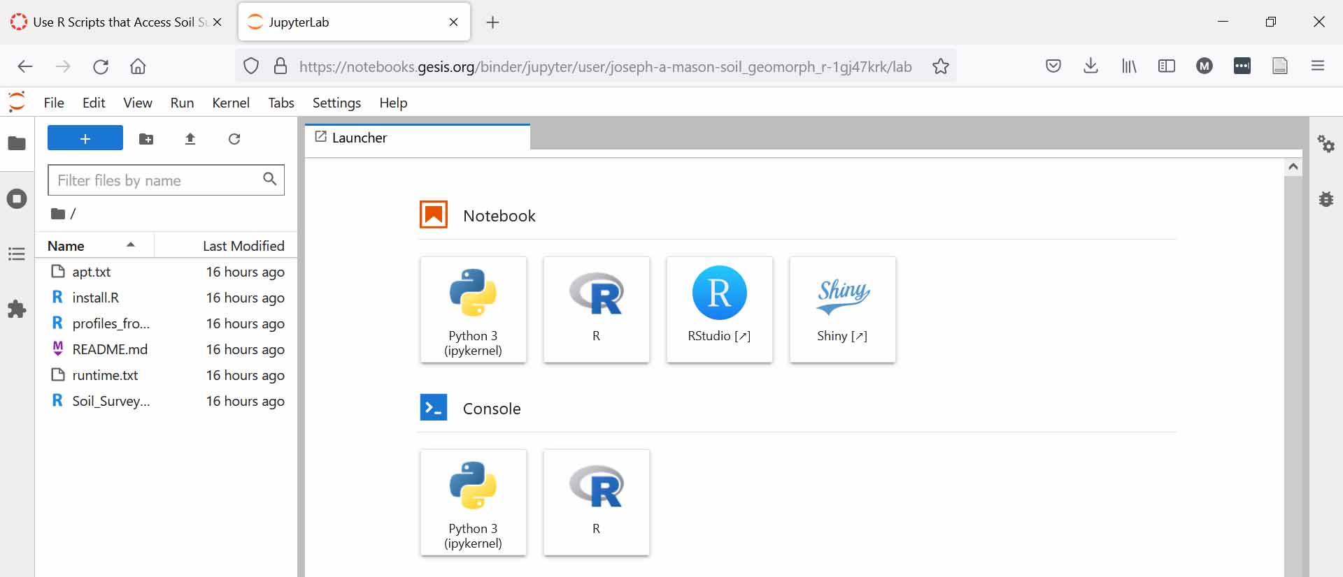

Click the button for RStudio (not one of the two R buttons). The RStudio interface should then appear. It should like what you see below, including the small window in the lower right with Files selected (I’ve added the red circle to show where it is). You should see a list of files there, including three __.R files. Of these, two are the scripts you can run (I’ve added stars by them).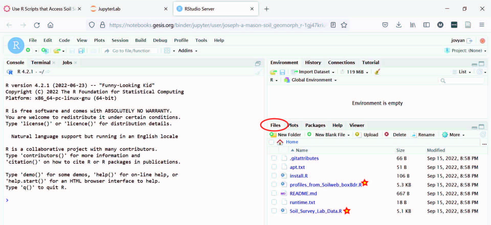

Click on either of these two R files and it will open in a new window in the upper left. Now you just need to run the script. First, though, take a look at it. All lines that start with ‘# or ##’ are comments, not R code. They usually explain what the code just below them does. They also alert you to where you can make changes in the code to look at different areas of the US or different soil series. Lines that start without ‘# or ##’ are the actual code that RStudio will run. You may want to look through the script and read the comments before running it.

To run the script, use the Run button just above it. You can do this in two ways 1) just keep clicking Run and it will work through the script, line by line, skipping the comments; or 2) select as much as you want to run at a time, or just the whole script, and click Run. Running blocks of code one by one allows you to relate what you see as output to the comments on that part of the script. Parts of the script do have to be run in the order listed in many cases and you can get errors if you run a later part without running something that comes earlier.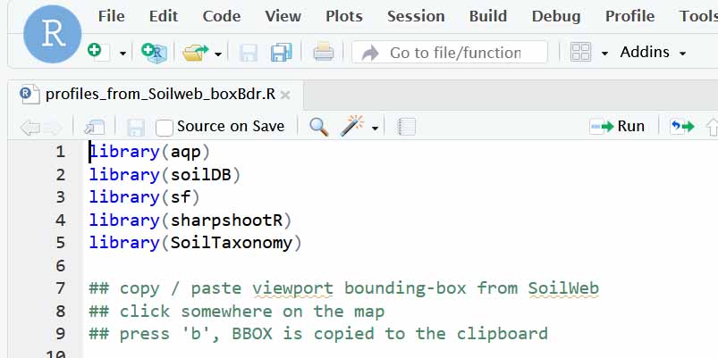

Plots produced by each script appear on the Plots tab in the lower right window</strong> (where you initial found the R scripts under the Files tab). You may need to select the Plots tab to see them. Only the last plot produced will be visible but you can page back and forth between them using the two arrows in the top right of the Plots tab. The plots will look bad, crowded together, in the small window. Just click on the Zoom button and a correctly sized, much better-looking version will pop up.

Final notes: Nothing you do in this notebook is saved, once you close it. Copy and past anything you want to keep into another document. If you want to install RStudio on your computer, I can give you advice on how to do it. For one thing, you will need to also install all of the R packages each script opens (the list of library(—) lines at the top). This can get complicated because of version issues. The scripts are available here: https://github.com/Joseph-A-Mason/soil_geomorph_r; you don’t need any of the other files there. RStudio is freely available (for the version we need).

To cite aqp in publications use:

Beaudette, D., Roudier, P., Brown, A. (2022). aqp: Algorithms for
Quantitative Pedology. R package version 1.42.
https://CRAN.R-project.org/package=aqp

Beaudette, D.E., Roudier, P., O'Geen, A.T. Algorithms for
quantitative pedology: A toolkit for soil scientists, Computers &
Geosciences, Volume 52, March 2013, Pages 258-268, ISSN 0098-3004,
http://dx.doi.org/10.1016/j.cageo.2012.10.020